Electric permittivity is one of the fundamental properties of a material, serving as a core concept in electromagnetics. While it is often treated as a real-valued constant, this simplified approach cannot be applied to most practical materials. In fact, a material's permittivity generally turns out to be a frequency-dependent complex quantity. In this article, we explore the concept of complex permittivity and its physical consequences.
Dielectric as an LTI System
Under an applied electric field, a dielectric material becomes polarized. The degree of this polarization is represented by the polarization density ${\bf P}({\bf x}, t)$, defined as the dipole moment per unit volume: ${\bf P} = \frac{\Delta {\bf p}}{\Delta V}$. This relationship, where the electric field ${\bf E}({\bf x}, t)$ results in a polarization density ${\bf P}({\bf x}, t)$ of a dielectric, can be viewed as a system accepting ${\bf E}$ as the input and, in response, producing ${\bf P}$ as the output.
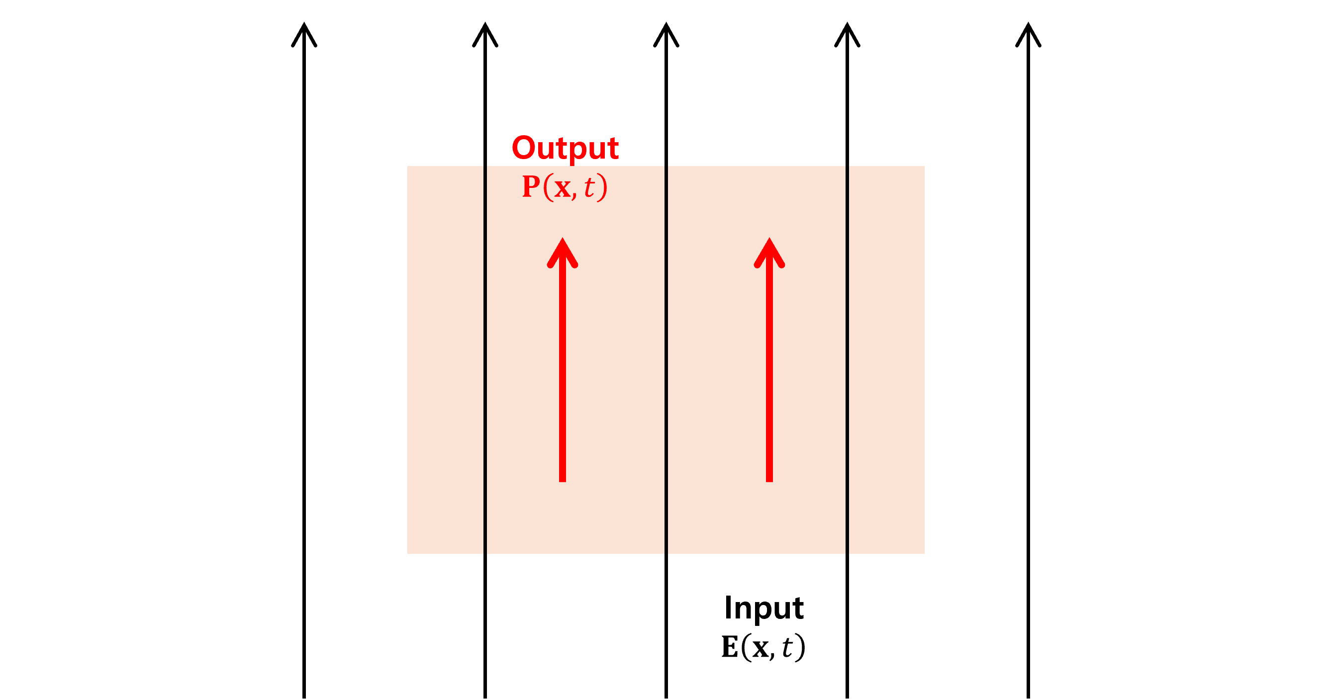
Figure 1 Dielectric as a system. The dielectric (orange-shaded area) accepts the electric field $\mathbf{E}$ as the input and, in response, produces the polarization density $\mathbf{P}$ as the output.
Moreover, it is often modeled as an LTI system, satisfying:
(i) Time Invariance. If ${\bf E}({\bf x}, t) \xrightarrow{\mathcal{D}} {\bf P}({\bf x}, t)$, then ${\bf E}({\bf x}, t-T) \xrightarrow{\mathcal{D}} {\bf P}({\bf x}, t-T)$.
(ii) Linearity. If ${\bf E}_1({\bf x}, t) \xrightarrow{\mathcal{D}} {\bf P}_1({\bf x}, t)$ and ${\bf E}_2({\bf x}, t) \xrightarrow{\mathcal{D}} {\bf P}_2({\bf x}, t)$, then $a{\bf E}_1({\bf x}, t) \xrightarrow{\mathcal{D}} a{\bf P}_1({\bf x}, t)$ and ${\bf E}_1({\bf x}, t)+{\bf E}_2({\bf x}, t) \xrightarrow{\mathcal{D}} {\bf P}_1({\bf x}, t)+{\bf P}_2({\bf x}, t)$.
Here, the mapping from input to output is denoted by the arrow $\xrightarrow{\mathcal{D}}$, where $\mathcal{D}$ represents the dielectric system. While time invariance is a reasonable condition, linearity isn't quite as intuitive. In fact, under high-intensity fields, the linearity condition breaks down. This phenomenon is studied in the field of nonlinear optics. However, we will assume linearity holds true throughout this article.
The input-output relationship of an LTI system can be expressed using its impulse response function, which is the output corresponding to a Dirac delta input $\delta(t)$. By writing the impulse response function of the system $\mathcal{D}$ as $\varepsilon_0 \chi(t)$, the relationship between the input ${\bf E}({\bf x}, t)$ and the output ${\bf P}({\bf x}, t)$ is given as a convolution:
$${\bf P}({\bf x}, t) = \varepsilon_0 \int_{-\infty}^{+\infty}{\chi(t-t^\prime){\bf E}({\bf x}, t^\prime)dt^\prime}$$
Note that the isotropy of the dielectric is implicitly assumed by writing the impulse response function as a scalar $\epsilon_0 \chi(t)$, rather than a 3 by 3 tensor, even though the input and the output of the system are 3-component vectors.$^1$
Furthermore, the system must be causal, which requires $\chi(t)=0$ for $t<0$, leading to:
$${\bf P}({\bf x}, t) = \varepsilon_0 \int_{-\infty}^{t}{\chi(t-t^\prime){\bf E}({\bf x}, t^\prime)dt^\prime}$$
It is natural to take a look at the Fourier domain, where the convolution turns into a straightforward multiplication. In the Fourier domain, the relationship between the input and the output is expressed as:
$${\bf P}({\bf x}, \omega) = \varepsilon_0 \chi(\omega){\bf E}({\bf x}, \omega)$$
Where ${\bf P}({\bf x}, \omega)$, ${\bf E}({\bf x}, \omega)$, $\chi(\omega)$ are the Fourier transforms of ${\bf P}({\bf x}, t)$, ${\bf E}({\bf x}, t)$, $\chi(t)$, respectively:
$${\bf P}({\bf x}, \omega) = \frac{1}{2\pi} \int_{-\infty}^{+\infty}{{\bf P}({\bf x}, t)e^{-i\omega t}dt} \\ {\bf E}({\bf x}, \omega) = \frac{1}{2\pi} \int_{-\infty}^{+\infty}{{\bf E}({\bf x}, t)e^{-i\omega t}dt} \\ \chi(\omega) = \frac{1}{2\pi} \int_{-\infty}^{+\infty}{\chi(t)e^{-i\omega t}dt}$$
Recall that the electric displacement field $\bf D$ is defined as ${\bf D}({\bf x}, t) = \varepsilon_0 {\bf E}({\bf x}, t) + {\bf P}({\bf x}, t)$. Taking the Fourier transform of both sides of the equation, we obtain:
$$\begin{aligned} {\bf D}({\bf x}, \omega) &= \varepsilon_0 {\bf E}({\bf x}, \omega) + {\bf P}({\bf x}, \omega) \\ &= \varepsilon_0 (1+\chi(\omega)) {\bf E}({\bf x}, \omega) \\ &= \varepsilon (\omega) {\bf E}({\bf x}, \omega) \end{aligned}$$
Here, $\varepsilon(\omega)$ is defined as $\varepsilon(\omega) := \varepsilon_0 (1 + \chi(\omega))$. Since the Fourier transform of a function can be interpreted as the amplitude of its component oscillating as $e^{i\omega t}$, $\varepsilon(\omega)$ can be viewed as the frequency-dependent permittivity of the dielectric, defining the ratio between the $e^{i\omega t}$ components of the $\bf E$ and $\bf D$ fields.
Because $\chi (\omega)$ is the Fourier transform of the real-valued function $\chi (t)$, it is generally a complex quantity (to be precise, the function $\chi (\omega)$ is a Hermitian function, meaning $\chi(-\omega) = \chi^*(\omega)$), and so is the permittivity $\varepsilon (\omega)$.
For $\varepsilon(\omega)$ and $\chi(\omega)$ to be real, $\chi(t)$ needs to be Hermitian, which in conjunction with the causality condition ($\chi(t)=0$ for $t<0$), restricts $\chi(t)$ to be exactly zero everywhere except at $t=0$. This means the system has to respond to an input instantaneously: the output ${\bf P}({\bf x}, t)$ should be proportional to the input ${\bf E}({\bf x}, t)$ at every moment.
Concluding the discussion above, complex-valued permittivity is nothing special - it simply indicates that the response of the dielectric to an electric field is not instantaneous, resulting in a phase mismatch between the $e^{i\omega t}$ oscillating components of $\bf E$ and $\bf D$ fields.
The Origin of Complex Permittivity: The Lorentz Model
The frequency-dependent permittivity $\varepsilon(\omega)$ of a dielectric is effectively described using the Lorentz model. In this model, the bound charges of a dielectric are modeled as electrons bound to a stationary nucleus by a hypothetical spring with damping forces. The equation of motion for an electron at displacement ${\bf x}(t)$ from the nucleus, under a driving force originating from the applied electric field ${\bf E}(t)$, is given as:
$$\ddot{\bf x} + \gamma \dot{\bf x} + \omega_0^2 {\bf x} = -\frac{e}{m}{\bf E}(t)$$
Taking the Fourier transform of both sides of the equation yields:
$$(i\omega)^2 {\bf x}(\omega) + \gamma(i\omega){\bf x}(\omega) + \omega_0^2 {\bf x}(\omega) = -\frac{e}{m}{\bf E}(\omega)$$
or
$${\bf x}(\omega) = \frac{-\frac{e}{m}{\bf E}(\omega)}{(\omega_0^2-\omega^2) + i\gamma \omega}$$
Using the electron number density $N$, the polarization density ${\bf P}$ is calculated as ${\bf P} = N(-e{\bf x})$. Thus, we obtain:
$${\bf P}(\omega) = \frac{\frac{Ne^2}{m}}{(\omega_0^2-\omega^2) + i\gamma \omega}{\bf E}(\omega)$$
Comparing this result with ${\bf P}(\omega) = \varepsilon_0 \chi(\omega) {\bf E}(\omega)$ and $\varepsilon (\omega) = \varepsilon_0 (1 + \chi(\omega))$, we get:
$$\varepsilon(\omega) = \varepsilon_0 \left( 1 + \frac{Ne^2}{m\varepsilon_0} \frac{1}{(\omega_0^2-\omega^2) + i\gamma \omega} \right)$$
This simple model confirms the existence of an imaginary part of permittivity. Employing the definition of the plasma frequency $\omega_p = \sqrt{\frac{Ne^2}{m\varepsilon_0}}$, the relative permittivity $\varepsilon_r (\omega) = \frac{\varepsilon(\omega)}{\varepsilon_0}$ can be expressed as:
$$\varepsilon_r (\omega) = 1 + \frac{\omega_p^2}{(\omega_0^2-\omega^2) + i\gamma \omega} = \varepsilon_r' - i\varepsilon_r''$$
Here, $\varepsilon_r'$ and $\varepsilon_r''$ denote the real and imaginary parts of the relative permittivity, respectively.
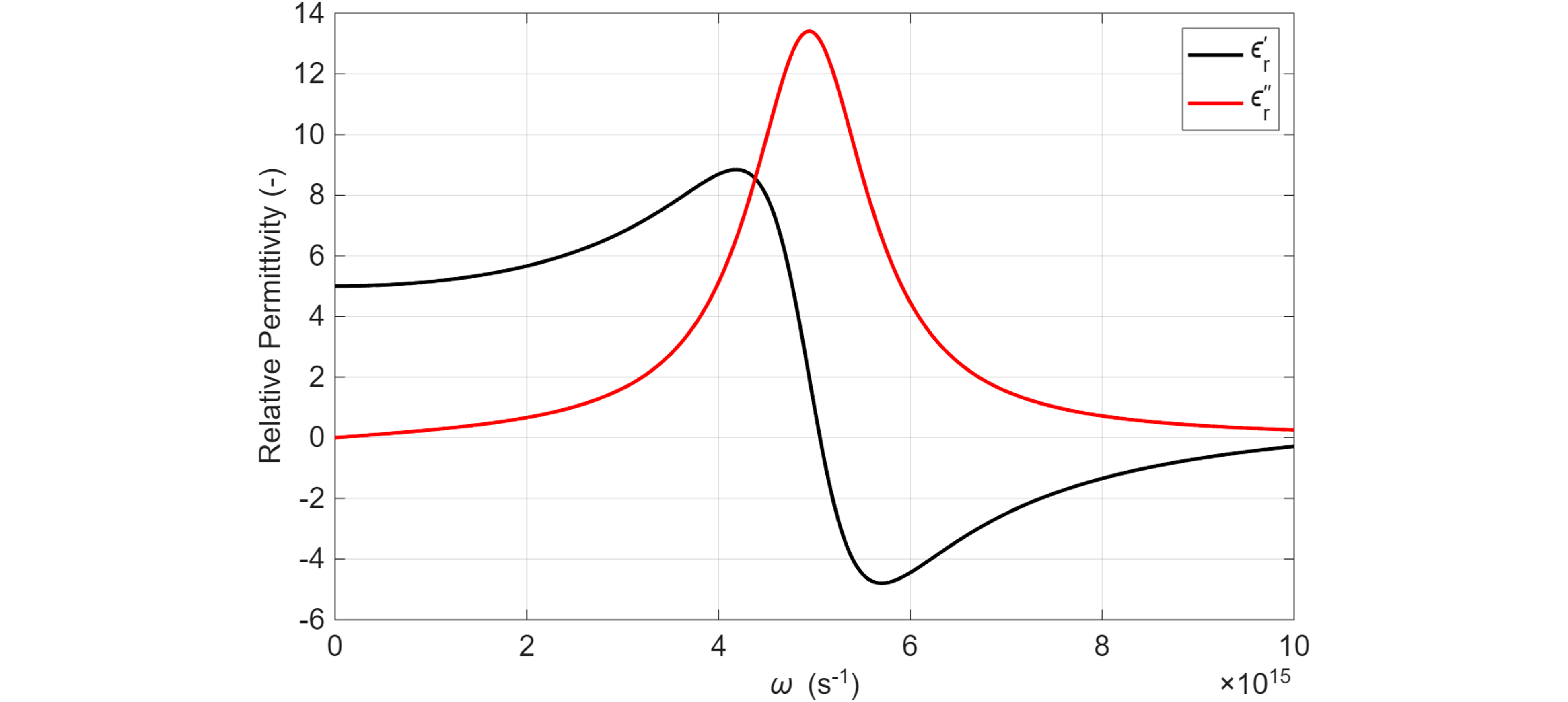
Figure 2 The real (black) and imaginary (red) parts of the frequency-dependent complex relative permittivity, derived from the Lorentz model. The parameters for the model are arbitrarily chosen as $\omega_p=1.0 \times 10^{16} {\rm \ rad/s}$, $\omega_0=5.0 \times 10^{15} {\rm \ rad/s}$, and $\gamma = 1.5 \times 10^{15} \ {\rm rad/s}$. Resonant behavior is clearly observed near the resonance $\omega = \omega_0$.
In practice, the Lorentz model is modified to account for multiple resonant frequencies:
$$\varepsilon_r = \varepsilon_\infty + \omega_p^2 \sum_j {\frac{f_j}{(\omega_{0,j}^2-\omega^2) + i\gamma_j \omega}}$$
where $\omega_{0,j}$ represents the distinct resonant frequencies arising from various absorption mechanisms within the material, while $f_j$ and $\gamma_j$ denote their corresponding oscillator strengths and damping coefficients.
Conductivity as Effective Permittivity
However, this is not the only reason for complex values of permittivity. So far we have only considered the effect of the bound charges. Yet some dielectric materials, and metals in the extreme, have charges that are unbound and travel freely, contributing to free currents. The effect of this free current can be included in the definition of permittivity to construct the effective permittivity.
To elaborate on this idea, we start with the complete form of Maxwell's equations:
$$\begin{cases} \nabla \cdot {\bf D}({\bf x}, t) = \rho_f({\bf x}, t) \\ \nabla \cdot {\bf B}({\bf x}, t) = 0 \\ \nabla \times {\bf E}({\bf x}, t) = - \frac{\partial {\bf B}({\bf x}, t)}{\partial t} \\ \nabla \times {\bf H}({\bf x}, t) = {\bf J}_f({\bf x}, t) + \frac{\partial {\bf D}({\bf x}, t)}{\partial t} \end{cases}$$
Applying the Fourier transform to these equations yields:
$$\begin{cases} \nabla \cdot {\bf D}({\bf x}, \omega) = \rho_f({\bf x}, \omega) \\ \nabla \cdot {\bf B}({\bf x}, \omega) = 0 \\ \nabla \times {\bf E}({\bf x}, \omega) = - i\omega {\bf B}({\bf x}, \omega) \\ \nabla \times {\bf H}({\bf x}, \omega) = {\bf J}_f({\bf x}, \omega) + i\omega {\bf D}({\bf x}, \omega) \end{cases}$$
The conductivity $\sigma$ of the material defines the relation between the free current and the electric field as ${\bf J}_f = \sigma {\bf E}$. Substituting this equation into the Maxwell-Ampere law (the 4th equation), we obtain:
$$\begin{aligned} \nabla \times {\bf H}({\bf x}, \omega) = {\bf J}_f({\bf x}, \omega) + i\omega {\bf D}({\bf x}, \omega) &= \sigma {\bf E}({\bf x}, \omega) + i\omega {\bf D}({\bf x}, \omega) \\ &= \sigma {\bf E}({\bf x}, \omega) + i\omega\varepsilon {\bf E}({\bf x}, \omega) \\ &= i\omega \left( \varepsilon - i \frac{\sigma}{\omega} \right) {\bf E}({\bf x}, \omega) \\ &= i\omega \hat{\varepsilon} {\bf E}({\bf x}, \omega) \end{aligned}$$
Thus, we define $\hat{\varepsilon} := \varepsilon - i\frac{\sigma}{\omega}$ as the effective permittivity, which absorbs the effect of conductivity as the imaginary part of the permittivity.
One might wonder if replacing the original permittivity with the effective permittivity is consistent with the other Maxwell's equations. The only relation that needs to be examined is Gauss's law (the 1st equation), substituting ${\bf D}$ with $\hat{\bf D} = \hat{\varepsilon}{\bf E}$. Starting from $\nabla \times {\bf H}({\bf x}, \omega) = i\omega \hat{\varepsilon} {\bf E}({\bf x}, \omega)$, we get:
$$\nabla \cdot \hat{\bf D} = \nabla \cdot \left(\hat{\varepsilon}{\bf E}\right) = \frac{1}{i\omega} \nabla \cdot \left( \nabla \times {\bf H} \right) = 0$$
Thus, setting $\hat{\rho}_f = 0$ as well as $\hat{\bf J}_f = 0$ yields the following consistent set of Maxwell equations:
$$\begin{cases} \nabla \cdot \hat{\bf D}({\bf x}, \omega) = 0 \\ \nabla \cdot {\bf B}({\bf x}, \omega) = 0 \\ \nabla \times {\bf E}({\bf x}, \omega) = - i\omega {\bf B}({\bf x}, \omega) \\ \nabla \times {\bf H}({\bf x}, \omega) = i\omega \hat{\bf D}({\bf x}, \omega) \end{cases}$$
where $\hat{\bf D} = \hat{\varepsilon}{\bf E}$.
In other words, solving Maxwell's equations for a dielectric with conductivity $\sigma$, in which nonzero free charge and free current can exist, is equivalent to solving those for a new dielectric which precludes free charge or current, using the modified effective permittivity of $\hat{\varepsilon} = \varepsilon - i\frac{\sigma}{\omega}$.
A lot of literature presents the value of this effective permittivity simply as "the permittivity" without clarification. Because of this, the conductivity of a material is often an important component of the reported complex permittivity value. Nonetheless, it must be emphasized that this component does not account for the material's true polarization density ${\bf P}$, which is strictly defined by the dipole moments of the bound charges, in response to the to the electric field ${\bf E}$.
The Consequences of Complex Permittivity
Summarizing the discussion in the section above, Maxwell's equations in the Fourier domain are given as:
$$\begin{cases} \nabla \cdot {\bf D}({\bf x}, \omega) = 0 \\ \nabla \cdot {\bf B}({\bf x}, \omega) = 0 \\ \nabla \times {\bf E}({\bf x}, \omega) = - i\omega {\bf B}({\bf x}, \omega) \\ \nabla \times {\bf H}({\bf x}, \omega) = i\omega {\bf D}({\bf x}, \omega) \end{cases}$$
Here, ${\bf D} = \varepsilon {\bf E}$ represents either the original displacement field in a non-conductive ($\sigma = 0$) dielectric medium, or the effective displacement field defined with the effective permittivity $\varepsilon$ that includes the conductivity term, in a conductive (finite $\sigma$) dielectric medium. In either case, the permittivity $\varepsilon(\omega)$ is fundamentally a complex value.
Starting from these equations, we obtain the equations for the propagation of electromagnetic waves in a dielectric medium. Specifically, the curl operator $\nabla \times$ is applied to both sides of Faraday's law to get:
$$ \nabla \times \left( \nabla \times {\bf E}({\bf x}, \omega) \right) = -i\omega \nabla \times {\bf B}({\bf x}, \omega) $$
The left-hand side is simplified using the vector identity:
$$\nabla \times \left( \nabla \times {\bf E}({\bf x}, \omega) \right) = \nabla \left( \nabla \cdot {\bf E} \right) - \nabla^2 {\bf E} = \frac{1}{\varepsilon} \nabla \left( \nabla \cdot {\bf D} \right) - \nabla^2 {\bf E} = - \nabla^2 {\bf E}({\bf x}, \omega)$$
Although not explicitly discussed in this article, the ${\bf H}$ field and the ${\bf B}$ field are related in the same manner as the electric fields: ${\bf B}({\bf x}, \omega) = \mu {\bf H}({\bf x}, \omega)$. Moreover, in most materials of interest, the approximation $\mu \approx \mu_0$ is valid. Using this fact with the Maxwell-Ampere law, the right-hand side is calculated as:
$$-i\omega \nabla \times {\bf B}({\bf x}, \omega) = -i\omega \mu_0 \nabla \times {\bf H} = \omega^2 \mu_0 {\bf D} = \omega^2 \mu_o \varepsilon {\bf E}({\bf x}, \omega) = k^2 {\bf E}({\bf x}, \omega)$$
where $k = k' - ik'' := (\omega^2 \mu_0 \varepsilon)^\frac{1}{2}$ is the complex wavenumber.
Therefore, the equation for electromagnetic wave propagation is derived in the form of the Helmholtz equation:
$$\nabla^2 {\bf E}({\bf x}, \omega) + k^2 {\bf E}({\bf x}, \omega) = 0 $$
This equation has the plane wave solution:
$${\bf E}({\bf x}, \omega) = {\bf A}(\omega)e^{-i {\bf k} \cdot {\bf x}}, \ |{\bf k}|=k$$
or, in the time domain,
$${\bf E}({\bf x}, t) = \int_{-\infty}^{+\infty} {{\bf A}(\omega)e^{i(\omega t - {\bf k} \cdot {\bf x})}d\omega}$$
The resultant field oscillates as $e^{-i {\bf k}\cdot {\bf x}}$ in the spatial dimension. Assuming the direction of propagation as the +z-direction without loss of generality, we notice that:
$$e^{-i {\bf k} \cdot {\bf x}} = e^{-ikz} = e^{-i(k' - ik'')z} = e^{-k'' z}e^{-ik' z}$$
This means that the field is attenuated according to $e^{-k'' z}$ while oscillating as $e^{-ik' z}$. For this reason, the imaginary part $k''$ of the complex wavenumber $k$ is called the attenuation constant, while the real part $k'$ is called the phase constant.
It is worth noting that the imaginary part of $k$ arose because the permittivity $\varepsilon$ is complex, since the two are related as $k = (\omega^2 \mu_0 \varepsilon)^\frac{1}{2}$. Recalling that in the Lorentz model, the imaginary part of the permittivity comes from the damping coefficient $\gamma$ of electrons, the fact that the imaginary part of the wavenumber leads to the attenuation of the field is not surprising.
Meanwhile, the complex refractive index can also be defined using the complex wavenumber, as:
$$\tilde{n} = n-i\kappa := \frac{ck}{\omega}$$
The imaginary part $\kappa$ is called the extinction coefficient, while the real part $n$ is often simply referred to as the refractive index. From the above definition, the relationship between the complex refractive index and the complex permittivity can be derived as follows:
$$\tilde{n} = \frac{ck}{\omega} = \frac{c}{\omega}(\omega^2 \mu_0 \varepsilon)^\frac{1}{2} = \frac{(\mu_0 \varepsilon)^{\frac{1}{2}}}{(\mu_0 \varepsilon_0)^{\frac{1}{2}}} = \varepsilon_r^{\frac{1}{2}}$$
The real and imaginary parts of $\tilde{n}$ and $\varepsilon_r$ are related as:
$$\varepsilon_r' = n^2 - \kappa^2 \\ \varepsilon_r'' = 2n\kappa$$
The refractive index $n$ and the extinction coefficient $\kappa$ of a material can be experimentally measured by spectroscopic ellipsometry.
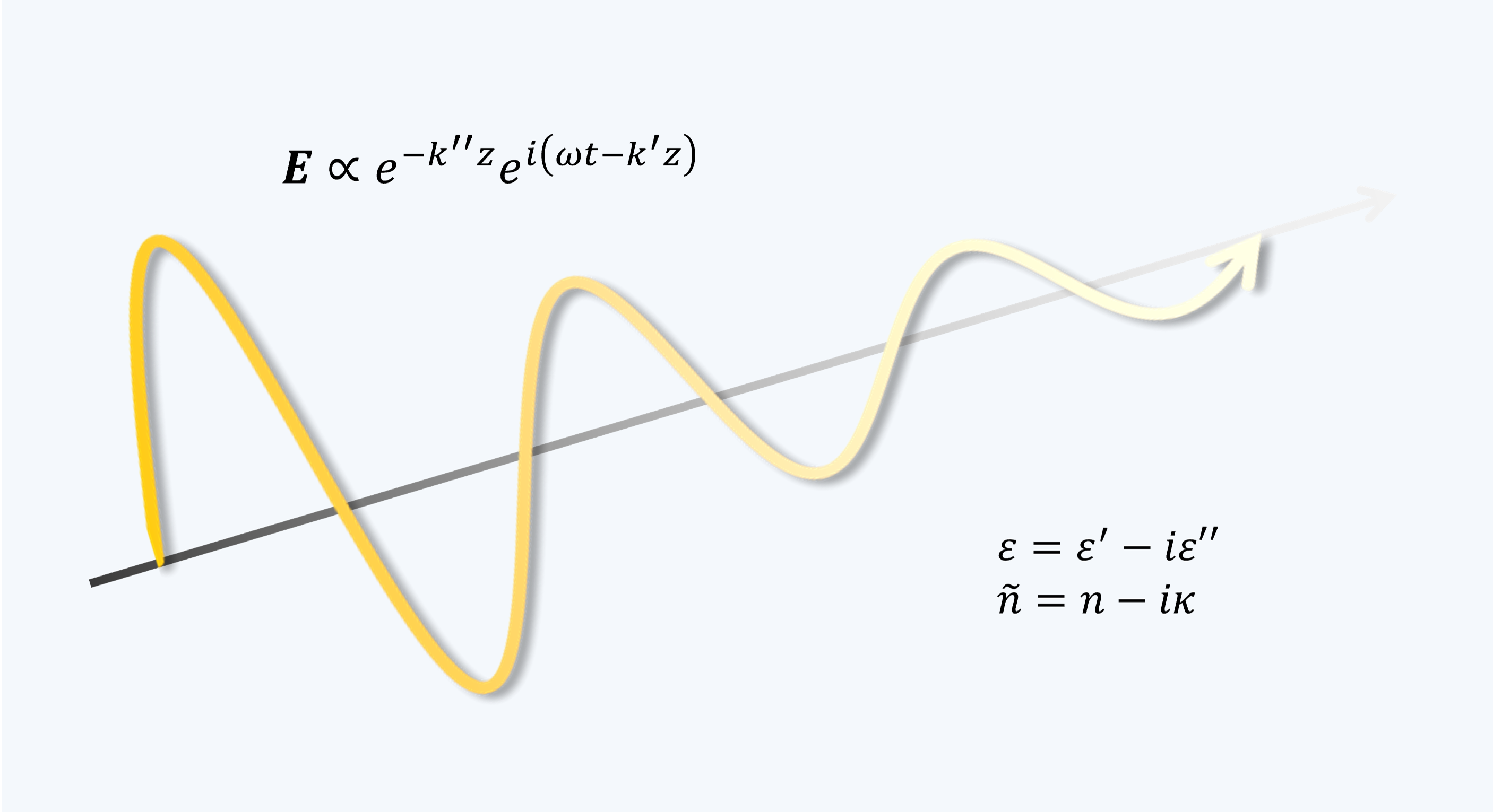
Figure 3 Propagation of an electromagnetic field in a medium. The field is attenuated as it propagates due to the imaginary component of the permittivity.
$^1$ For an anisotropic material, the relationship between $\mathbf{E}$ and $\mathbf{P}$ should be expressed as: $$P_i({\bf x}, t) = \varepsilon_0 \int_{-\infty}^{+\infty}{\sum_j\chi_{ij}(t-t^\prime)E_j({\bf x}, t^\prime)dt^\prime}$$