Diffraction Formula in Scalar Diffraction Theory

Figure 1 Coordinate system for scalar diffraction theory. An input electromagnetic wave, denoted as $U(\xi,\eta)$, propagates along the $z$-direction through free space to form the output wave $U(x,y)$.

According to scalar diffraction theory, an input electromagnetic wave at the $z=0$ plane, $U(\xi, \eta)$, propagates through free space to form the output wave at the $z=z$ plane, $U(x,y)$, as follows:

$$U(x,y) = \frac{z}{j\lambda}\iint{U(\xi,\eta) \frac{\exp{\left( jk\sqrt{(x-\xi)^2+(y-\eta)^2+z^2} \right)}}{(x-\xi)^2+(y-\eta)^2+z^2}}d\xi d\eta$$

This is the first Rayleigh-Sommerfeld diffraction formula.

The Fresnel diffraction formula for the near field approximation is obtained by assuming $|x-\xi| \ll z$ and $|y-\eta| \ll z$, which allows $\sqrt{(x-\xi)^2+(y-\eta)^2+z^2}\approx z + \frac{(x-\xi)^2+(y-\eta)^2}{2z}$. The resultant formula is:

$$\begin{aligned} U(x,y) &= \frac{e^{jkz}}{j\lambda z}\iint U(\xi,\eta) \exp{\left[ j \frac{\pi}{\lambda z}((x-\xi)^2 + (y-\eta)^2) \right]}d\xi d\eta \\ &= \frac{e^{jkz}}{j\lambda z} \exp{\left[ j \frac{\pi}{\lambda z}(x^2 + y^2) \right]} \mathcal{F} \left\lbrace U(\xi,\eta)\exp{\left[ j \frac{\pi}{\lambda z}(\xi^2 + \eta^2) \right]} \right\rbrace_{f_\xi = \frac{x}{\lambda z}, \ f_\eta = \frac{y}{\lambda z}} \end{aligned}$$

Here $\mathcal{F}$ denotes the Fourier transform. This formula can be further approximated, for the far field pattern, by assuming $z \gg \frac{k(\xi^2 + \eta^2)}{2}$, which gives $\exp{\left[ j\frac{\pi}{\lambda z}(\xi^2 + \eta^2) \right]} \approx 1$. This is called the Fraunhofer diffraction formula:

$$U(x,y) = \frac{e^{jkz}}{j\lambda z} \exp{\left[ j \frac{\pi}{\lambda z}(x^2 + y^2) \right]} \mathcal{F} \left\lbrace U(\xi,\eta) \right\rbrace_{f_\xi = \frac{x}{\lambda z}, \ f_\eta = \frac{y}{\lambda z}}$$

Talbot Images

Figure 2 Input wave pattern for the Talbot effect, overlaid on the coordinate axes. The red lines correspond to the peaks of the sinusoidal input wave.

Talbot images are an interesting phenomenon that arises in near field patterns. Assume a periodic input of $U(\xi, \eta) = \frac{1}{2} \left[ 1 + m \cos\left(\frac{2\pi \xi}{L}\right) \right]$. Substituting this input pattern into the Fresnel diffraction formula, we obtain:

$$|U(x,y)|^2 = \frac{1}{4}\left[ 1 + 2m \cos \left( \frac{\pi \lambda z}{L^2} \right) \cos \left(\frac{2\pi x}{L}\right) + m^2 \cos^2 \left(\frac{2\pi x}{L}\right) \right]$$

At $z = n\times\frac{2L^2}{\lambda}$ ($n=1,2,\dots$), this is simplified to:

$$|U(x,y)|^2 = \frac{1}{4}\left[1+m\cos \left(\frac{2\pi x}{L}\right)\right]^2$$

Since what we detect is the intensity of the field pattern, we can conclude that the same periodic image as the input repeatedly appears at locations $z = n\times\frac{2L^2}{\lambda}$. These are called the Talbot images.

Talbot Images in the Far Field?

However, in the far field, the Fraunhofer diffraction formula applied to the diffraction pattern of the input $U(\xi, \eta) = \frac{1}{2} \left[ 1 + m \cos\left(\frac{2\pi \xi}{L}\right) \right]$ gives:

$$U(x,y) \propto \left[\frac{1}{2}\delta(x) + \frac{m}{4}\delta\left(x-\frac{\lambda z}{L}\right) + \frac{m}{4}\delta\left(x+\frac{\lambda z}{L} \right)\right]\delta (y)$$

This means that the output field pattern consists of three dots at $(0,0)$, $(\frac{\lambda z}{L},0)$, and $(-\frac{\lambda z}{L},0)$, which is apparently distinct from the Talbot image pattern we derived earlier. Talbot images were predicted to appear every $\frac{2L^2}{\lambda}$ in the $z$-direction, yet they disappear when using the Fraunhofer diffraction formula. Where did the Talbot images go?

This mismatch is because the Fraunhofer diffraction formula is no longer a valid approximation for the Fresnel diffraction formula when given the $U(\xi, \eta) = \frac{1}{2} \left[ 1 + m \cos\left(\frac{2\pi \xi}{L}\right) \right]$ input pattern. While deriving the Fraunhofer diffraction formula from the Fresnel diffraction formula, we used the approximation $z \gg \frac{k(\xi^2 + \eta^2)}{2}$. Therefore, the input field pattern needs to be confined to a small region compared to the length of propagation. However, the input of $U(\xi, \eta) = \frac{1}{2} \left[ 1 + m \cos\left(\frac{2\pi \xi}{L}\right) \right]$ extends infinitely in the $z=0$ $(\xi,\eta)$-plane, introducing a non-negligible discrepancy between the Fresnel and Fraunhofer diffraction formulas.

In reality, the input field pattern does not extend to infinity in the $(\xi,\eta)$-plane. Instead, it is confined to a region near the origin. One way to model this reality is by multiplying the input by a rect function, which represents the finite size of the aperture:

$$U(\xi, \eta) = \frac{1}{2} \left[ 1 + m \cos\left(\frac{2\pi \xi}{L}\right) \right] \times {\rm rect}\left(\frac{\xi}{D}\right){\rm rect}\left(\frac{\eta}{D}\right) $$

This disruption causes the Talbot image pattern to fade away in the far field, and instead creates a three-dot pattern (more precisely, three sinc lobes) as expected by the Fraunhofer diffraction formula. Figure 3 shows the numerical calculation results for the propagation of this modified input according to the exact Rayleigh-Sommerfeld formula. Figure 3(b) illustrates the gradual evolution of the field pattern, from a Talbot image in the near field to a close-up bright point in the far field. The wide shot plot of the field pattern at the far field, depicted in Figure 3(c), clearly shows the three dots along the $x$-axis.

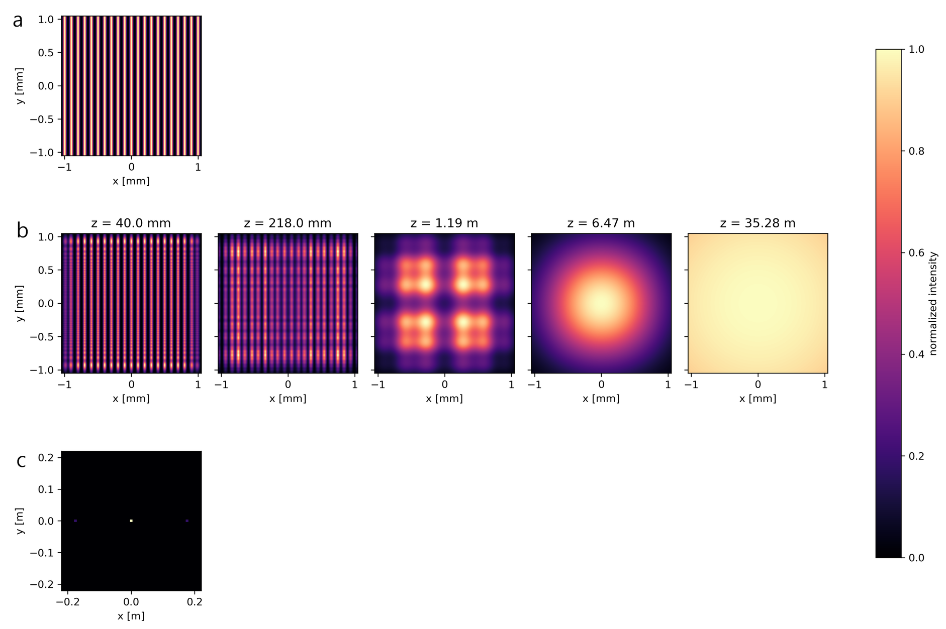
Figure 3 Numerical calculation results obtained using the Rayleigh-Sommerfeld formula for the propagation of the truncated sinusoidal input. (a) The input pattern. (b) The gradual evolution from a near field Talbot image to far field sinc lobes. (c) A wider view of the 5th panel in (b), showing the field pattern in the far field.