• Yildirim, M., Dinc, N.U., Oguz, I., Psaltis, D., Moser, C. Nonlinear processing with linear optics. Nat. Photon. 18, 1076–1082 (2024).

Introduction

Nonlinear activation is an essential component in neural networks to enable the representation of complex relationships between inputs and outputs.$^1$ This holds true not only for traditional neural networks powered by electronic computing, but also for optical neural networks (ONNs), which are an emerging field of research due to their high energy efficiency and computing speed. Consequently, there have recently been intensive studies on implementing nonlinear activation functions in ONNs.$^{2,3}$

One way to incorporate nonlinearity in ONNs is to exploit the nonlinear light-matter interactions inherent in nature. However, these types of optical nonlinear effects are usually weak, and therefore require strong field intensities, and ultimately, high power consumption, in order to obtain sufficient nonlinearity needed for practical performance.$^1$

This paper, published in Nature Photonics by Yildirim et al., attempts to address this problem of high power requirements for nonlinear activation in ONNs by proposing a nonlinear operation framework constructed solely with linear optics: nPOLO (nonlinear Processing with Only Linear Optics). To achieve this, the authors utilize structural nonlinearity. In this strategy, the linear transfer function of the system of interest is equipped with an input dependency, leading to a nonlinear relationship between the input and the output, instead of implementing a nonlinear transfer function itself.$^1$

Although the strategy of utilizing structural nonlinearity has been around from before$^{4,5}$, this paper is one of the first reports of experimentally implementing it at optical frequencies.$^{1,6,7,8}$ The results are particularly significant because the authors validate the performance of the constructed neural network by applying it to actual image classification datasets commonly used as benchmarks.

Methods

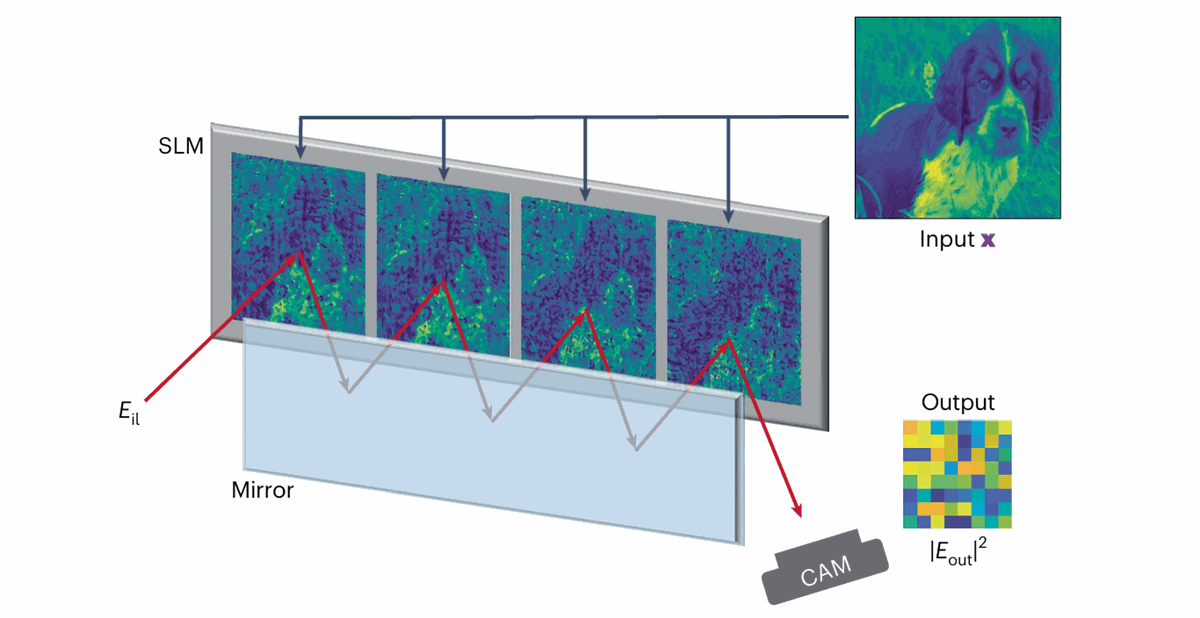
Figure 1 The optical setup for the nPOLO framework. Adapted from Figure 1 in the original paper.

The optical setup for the nPOLO framework consists of $N$ SLMs (Spatial Light Modulators), a mirror to guide the light path, a light source, and a detector. The number of SLMs, $N$, is referred to as the number of layers in this ONN system. As depicted in Figure 1, the incident light is modulated by the first SLM, reflected back by the mirror, and directed towards the second SLM. This process is repeated until the light reflects off all $N$ SLMs and is finally captured by the detector. The SLMs are evenly spaced, and the mirror is placed parallel to them, so the diffraction operators representing the propagation from one SLM to the adjacent one are all identically denoted by $H$. Additionally, each SLM displays signals that are dependent on the input to the ONN system, $\mathbf{x}$, so the transmittance (or, more practically, the reflectance) of the $n$-th SLM is represented as $T_{Ln} (\mathbf{x})$. The light captured by the detector, $E_{out}$, is calculated from the incident light, $E_{il}$, as follows:

$$E_{out} = HT_{LN}(\mathbf{x}) \cdots HT_{L2}(\mathbf{x}) HT_{L1}(\mathbf{x}) E_{il}$$

For this relationship of the ONN, between the input $\mathbf{x}$ and the output $E_{out}$, to be trainable, the transmittance $T_{Ln}(\mathbf{x})$ must contain trainable parameters. In order to clearly address the effect of these trainable parameters and the resultant nonlinearity on the input $\mathbf{x}$, the authors assume that the SLM transmittance is controlled by the following linear function of the input:

$$t_j^{(n)} = s_j^{(n)}x_j + b_j^{(n)}$$

Here, $t_j^{(n)}$ and $x_j$ represents the $j$-th pixel's transmittance at the $n$-th SLM and the $j$-th pixel's value of the input $\mathbf{x}$, respectively, and $s_j^{(n)}$ and $b_j^{(n)}$ are trainable parameters. Calculating the $i$-th component of $E_{out}$ for small values of $N$, we obtain:

$$ \begin{aligned} N=1 :& \quad (E_{out})_i = \sum_j h_{ij} \left( s_j^{(1)} x_j + b_j^{(1)} \right) \quad \cdots \quad \text{1st order in input } \mathbf{x} \\ N=2 :& \quad (E_{out})_i = \sum_j h_{ij} \left( s_j^{(2)} x_j + b_j^{(2)} \right) \left( \sum_k h_{jk} \left( s_k^{(1)} x_k + b_k^{(1)} \right) \right) \quad \cdots \quad \text{2nd order in input } \mathbf{x} \end{aligned} $$

Here, $h_{ij}$ denotes the components of the diffractive matrix $H$, and the incident light is set to $E_{il} = 1$. Upon iteration for a general $N$-layer system, the output of this ONN is expressed as an $N$-th order polynomial in $\mathbf{x}$, with its coefficients dependent on the trainable parameters $s_j^{(n)}$ and $b_j^{(n)}$. Therefore, by recalling the Taylor expansion, it becomes clear that the nPOLO framework can express any arbitrary nonlinear function, provided that the number of layers $N$ is sufficiently large.

Yet, the optical setup used for the experiment utilized phase-only SLMs, so the SLM transmittance is given by $t_j^{(n)} = e^{j\left(s_j^{(n)}x_j + b_j^{(n)}\right)}$ instead of the linear relationship proposed above. Accordingly, the actual output is expressed as an $N$-th order polynomial in the cosine of the input $\mathbf{x}$, rather than $\mathbf{x}$ itself.$^9$

The authors tested the nPOLO framework on image classification tasks. The input images were fed to the SLMs, and a digital linear classifier was connected to the output captured by the detector to acquire the final classification result. Three datasets, Fashion MNIST, Digit MNIST, and Imagenette, were each used for training and testing. In the training process, the trainable parameters were optimized in silico, meaning that a computer simulation replicating the optical system of nPOLO was utilized to determine the trainable parameters via backpropagation. For testing, the physical SLMs displayed signals calculated from these optimized parameters, and the results of the final digital classifier were read to evaluate the accuracy.

Increasing the number of layers (the number of SLMs) enables higher-order nonlinearity in the input-output relationhip of nPOLO, but it also increases the number of trainable parameters - in other words, the space-bandwidth product (SBP) of the system. Thus, the enhanced performance cannot be attributed solely to the augmented nonlinearity. To evaluate the specific contribution of the high-order nonlinearity synthesized by nPOLO, the authors conducted an ablation study. They constructed an nPOLO system without data repetition; that is, they removed the input dependence and left only a trainable bias for every SLM except the first one. This ablated nPOLO was compared to the standard nPOLO system with data repetition to confirm the role of the $N$-th order nonlinearity created by $N$ layers of input-dependent SLMs.

Results

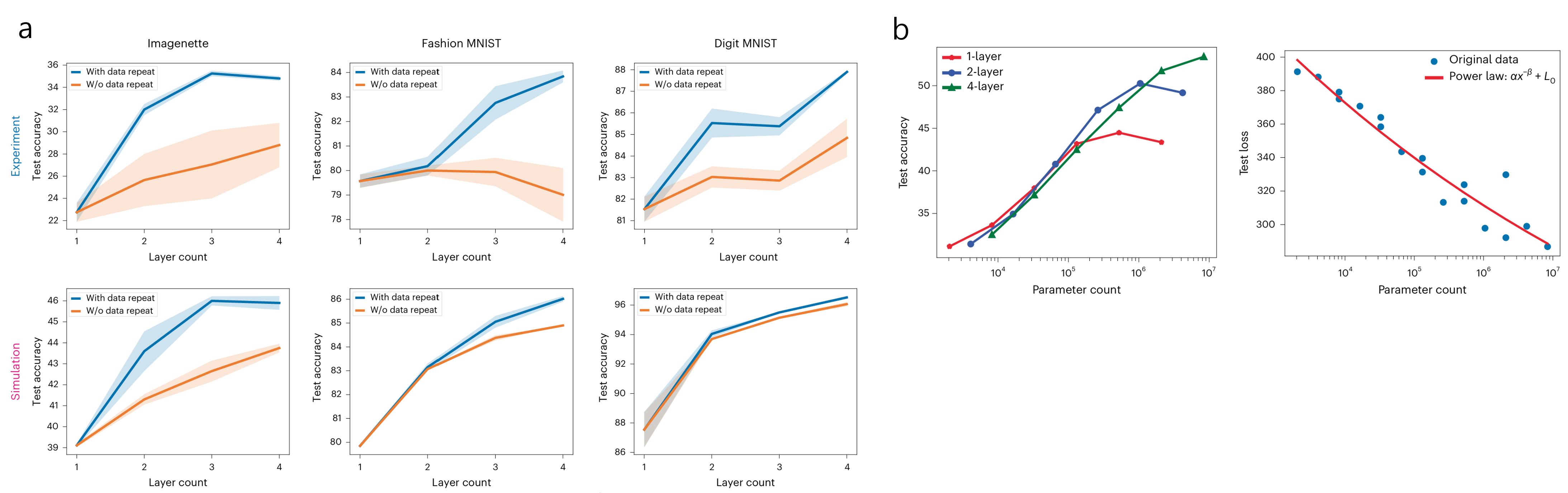
Figure 2 (a) Measured results of nPOLO performance. Each column shows the results for Imagenette, Fashion MNIST, and Digit MNIST, respectively. (b) Results of the scaling study. Adapted from Figure 2 and Figure 5 in the original paper, respectively.

The second row of Figure 2(a) shows the test accuracy calculated from the computer simulation by which in silico training was performed, while the first row shows the test accuracy evaluated using the physical optical system. In each graph, the blue line and the orange line represent the results of nPOLO with and without data repetition, respectively. Figure 2(b) illustrates the results of the scaling study, where the performances of various nPOLO systems with different numbers of trainable parameters were compared. The number of SLM pixels and the number of layers (SLMs) were varied to construct the diverse nPOLO systems plotted in the figure.

The main findings drawn by the authors from the experimental results are as follows:

(1) Data repetition enhances performance. The system with data repetition shows better performance compared to the system without it. This indicates that the high-order nonlinearity, implemented by the input dependence of each layer, contributes to performance improvement.

(2) Discrepancy exists between simulation and reality. The test accuracy measured with the physical optical setup is lower than that predicted by the simulation. The authors attribute this discrepancy to experimental errors in the actual SLMs. To support this, they inspected the performance change caused by introducing various experimental errors into the simulation, which showed that the performance robustness was improved for the system with data repetition. This coincides with the experimental observation that performance degradation is smaller when data repetition is present.

(3) Dataset complexity matters. The effect of data repetition is intensified for the more complex dataset (Imagenette). The authors explain that this is because the quadratic nonlinearity alone, which arises naturally when converting electromagnetic wave amplitude into detected intensity, is sufficient to learn simple datasets, making the high-order nonlinearity caused by data repetition unnecessary.

(4) Performance scales with parameters. The results of the scaling study show that performance scales with the total number of parameters, and this relationship is similar to the power-law relation recently reported for digital neural networks$^{10}$. Excessive parameters lead to performance saturation due to overfitting, and this point of saturation is delayed when the number of layers is increased to provide higher-order nonlinearity.

Comments

The authors demonstrated nPOLO, both theoretically and experimentally, as an implementation of nonlinear operation that utilizes only low-power linear optics by exploiting structural nonlinearity. The key contributions of this work are: (1) the authors assessed the performance of their system using standard datasets that are used as benchmarks for digital neural networks, and (2) they proved that the high-order nonlinearity synthesized by the multi-layer structure of their system genuinely enhances the performance, through a well-designed experiment comparing setups with and without data repetition.

However, this work also clearly illustrates the inherent limitation of optical (physical) neural networks that rely on in silico training: the mismatch between simulation and physical reality$^1$. The simulation and the actual optical system of nPOLO exhibited a considerable performance discrepancy, with the gap exceeding 10%p for test accuracy on the Imagenette dataset. This gap also contributes to the overall low performance of the nPOLO system. Current SOTA digital neural network models achieve over 90% accuracy on the Imagenet1K dataset (an extended version of the Imagenette dataset)$^{11}$, whereas the experimental accuracy of nPOLO on Imagenette was less than 40%. Notwithstanding the strengths of optical neural networks regarding energy consumption and computation speed, significant performance improvements are necessary for real-world applications. Physics-aware training$^{12}$ may be one way to address this problem. This method employs in silico simulations, but simultaneously incorporates feedback from the physical system to adjust the training. Since the training process reflects actual physical phenomena, the resulting trained model tends to attain higher performance.

$^1$ Abou-Hamdan, L. et al. Programmable metasurfaces for future photonic artificial intelligence. Nat. Rev. Phys. 7, 331–347 (2025).

$^{12}$ Wright, L. et al. Deep physical neural networks trained with backpropagation. Nature 601, 549-555 (2022).